
Tech and stuff
Tech and stuff
One of the first known uses of shortest path algorithms in technology was in telephony in the 1950’s. The problem was in finding alternate routing in case shortest route became blocked. In today’s world shortest path algorithms are used in plethora of applications. You can find them when calculating driving directions, airline travel routing, network communications, linguistics, social networks - they all use graphs to represent relationships between object.
In this particular post, I wanted to implement a weighed directed graph data structure. Because of its properties, weighed digraph is commonly used in mapping applications. I will use this graph in conjunction with the well-known Dijkstra’s algorithm to find shortest path between two points on a map. In order to do this, I will map intersection points on a small section of city map, then calculate shortest distance between those sets of points using our algorithm. Finally, I will use Google Maps driving directions on the same point sets to validate our experiment.
G = (V, E)
V - set of vertices; E - set of edges

Weighed directed graph also called weighed digraph is a graph containing a set of vertices (or nodes) connected by edges, where edges contain information about connection direction and the weight of that connection.
How does Dijkstra’s algorithms works? There’s a lot of good articles and videos explaining this relatively simple algorithm. I thought the video below does an excellent job at explaining it.
As you can see, Dijkstra’s algorithm is quite simple but it has some faults. In order to find shortest path between two vertices A and B, the algorithm has to visit all sub-graphs of the graph. With a large graph, this could be very time consuming. The good thing about Dijkstra’s algorithm is that once whole graph is scanned, we will have information about shortest path not only from vertex A to vertex B, but also to any vertex in the graph.
Below is the map I created based on a small section of Williamsburg in Brooklyn, NY. All circles represent graph vertices and the black lines with arrows are directed edges with assigned weights to each of them. Green circles will be our destination points.

Based on that map, I created an input file that will populate the graph with edges and vertices. We will use this file as an input data to our algorithm. Example data:
1 4 5.0
4 3 10.0
3 2 5.0
2 3 5.0
2 1 10.0
4 5 2.0
6 5 10.0
6 3 2.5
...
From the above example each row maps to the method of signature addEdge(from, to, weight)
Implementation of the graph will use adjacency-list approach to store information about edges. I tried to simplify code so it is easy to read, hence this is not an optimal implementation and it could definitely be improved upon.
https://github.com/markosski/shortestPath
Compile and run providing input file.
java DijkstraFind ../resources/map.txt
Running DijkstraFind should result in following output (representation of WeighedDigraph)
1 -> 4 @ 5.0,
2 -> 3 @ 5.0, 1 @ 10.0,
3 -> 2 @ 5.0, 6 @ 2.5,
4 -> 3 @ 10.0, 5 @ 2.0,
5 -> 7 @ 2.0, 8 @ 0.5, 13 @ 4.0,
6 -> 5 @ 10.0, 3 @ 2.5, 9 @ 3.0,
7 -> 13 @ 4.0,
8 -> 12 @ 2.0,
9 -> 8 @ 9.0, 6 @ 3.0, 11 @ 2.0,
10 -> 18 @ 2.0,
11 -> 9 @ 2.0, 10 @ 6.0, 17 @ 2.0,
12 -> 11 @ 9.5, 14 @ 1.0,
13 -> 14 @ 2.0,
14 -> 17 @ 8.0, 15 @ 0.5,
15 -> 21 @ 1.0,
17 -> 11 @ 2.0, 16 @ 4.0, 18 @ 6.0, 20 @ 2.0,
16 -> 14 @ 2.0, 15 @ 2.0,
19 -> 18 @ 2.0, 24 @ 2.0,
18 -> 17 @ 6.0, 10 @ 2.0, 19 @ 2.0,
21 -> 20 @ 6.0, 22 @ 2.0,
20 -> 17 @ 2.0, 19 @ 6.0, 23 @ 2.0,
23 -> 22 @ 5.0, 20 @ 2.0, 27 @ 2.0,
22 -> 28 @ 2.0,
25 -> 27 @ 6.0, 24 @ 2.0,
24 -> 23 @ 6.0, 19 @ 2.0, 25 @ 2.0,
27 -> 23 @ 2.0, 25 @ 6.0, 26 @ 4.0,
26 -> 27 @ 4.0,
28 -> 27 @ 2.5

Tests:
Test 1/Yellow: 4 -> 26: [4, 5, 8, 12, 14, 15, 21, 22, 28, 27, 26]
Test 2/Blue: 4 -> 19: [4, 5, 8, 12, 14, 15, 21, 20, 19]
Test 3/Green: 3 -> 28: [3, 6, 9, 11, 17, 20, 23, 22, 28]
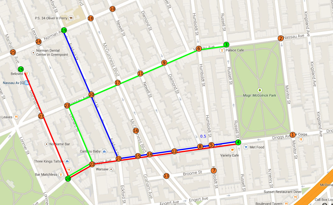 Result of Dijkstra’s algorithm directions
Now let’s see how well our algorithm performed comparing to Google Map directions. Below is the image with above results traced on the map. And here is Google Map results for the same origin -> destination sets.
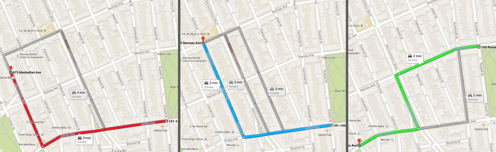 Result of Google Maps directions
As we can see, red and blue routes are exactly the same for our algorithm and Google Maps. Green directions however are a bit different than Google’s suggestions. Google Maps decided to take a left turn earlier for some reason, consequently adding slightly more distance to the route. Why is that? Well, this could be due to the fact we calculated our edge weights by using only distances between two points. In real life, edge weights would be a function of distance, speed limits, time of day, traffic conditions etc. Testing Google Maps at different time of day would likely yield different results because traffic patterns change throughout the day.
Here’s an interesting article from Microsoft that talks about research done on improving shortest path algorithm
Nice article explaining Dijkstra’s algorithm in more detail